Algorithm Complexity Analysis
Complexity Analysis is the practice of estimating the resources (primarily time and memory) an algorithm will consume relative to the size of its input. For a software developer, it is not just a theoretical concept; it is a fundamental tool for writing efficient, scalable, and performant code. Understanding complexity allows you to make informed decisions about which algorithm or data structure to use, and to anticipate how your application will behave as data volumes grow.
This guide focuses on the practical application of complexity analysis for software engineering, emphasizing intuition and real-world examples over formal mathematical proofs.
The Two Components of Complexity
Every algorithm consumes two main types of resources: Time and Space.
1. Time Complexity
- What it is: An estimation of the total number of operations an algorithm will perform as a function of its input size. It is not a measure of wall-clock time, but rather a measure of the algorithm’s growth rate. This makes it independent of the hardware it runs on.
- Why it matters: It helps predict how an algorithm will scale. An algorithm that is fast for 100 items might be unacceptably slow for 1 million items.
- Analogy: Imagine you have to read a book. Time complexity is not about how fast you can read (hardware speed), but about how the total reading time changes depending on the number of pages in the book (input size).
2. Space Complexity
- What it is: An estimation of the total memory an algorithm will use, including both the space taken by the inputs and any additional memory it allocates during execution (auxiliary space).
- Why it matters: In memory-constrained environments (like mobile or embedded systems) or with very large datasets, an algorithm with high space complexity can lead to crashes or poor performance.
- Analogy: While reading the book, space complexity is the number of sticky notes you need to use to keep track of characters and plot points. A simple story might need none (O(1) auxiliary space), while a complex one might require a note for every chapter (O(n) auxiliary space).
- Example (Recursion): A recursive function creates a new stack frame for each call. A function like
factorial(n)will makenrecursive calls before terminating, leading to a space complexity ofO(n)to store the call stack.
Asymptotic Notations & Case Analysis
Asymptotic notations are the language we use to describe an algorithm’s complexity as the input size () grows. This is typically analyzed in three main cases.
| Case | Notation | Purpose |
|---|---|---|
| Worst Case | O(f(n)) - Big-O | Upper Bound: Guarantees that the algorithm’s performance will not be worse than this. This is the most important case for developers. |
| Best Case | Ω(f(n)) - Big-Omega | Lower Bound: The fastest the algorithm can possibly run. |
| Average Case | Θ(f(n)) - Big-Theta | Tight Bound: The expected performance for a typical input. |
Little-o Notation (o)
- Purpose: Describes an upper bound that is not asymptotically tight.
- Meaning:
f(n) = o(g(n))means thatf(n)becomes insignificantly small compared tog(n)asnapproaches infinity. In simpler terms,f(n)grows strictly slower thang(n). - Analogy: If
g(n)is your maximum speed,o(g(n))means you’re driving at a speed that is always getting further and further below your maximum. - Example:
2n = o(n^2)because2ngrows strictly slower thann^2. However,2nis noto(n)because2ndoes not grow strictly slower thann(they grow at the same rate).
Little-omega Notation (ω)
- Purpose: Describes a lower bound that is not asymptotically tight.
- Meaning:
f(n) = ω(g(n))means thatf(n)becomes arbitrarily large compared tog(n)asnapproaches infinity. In simpler terms,f(n)grows strictly faster thang(n). - Analogy: If
g(n)is your minimum required speed,ω(g(n))means you’re driving at a speed that is always getting further and further above your minimum. - Example:
n^2 = ω(n)becausen^2grows strictly faster thann. However,n^2is notω(n^2)becausen^2does not grow strictly faster thann^2(they grow at the same rate).
Example: Searching an Array
Consider searching for an item in an array of size n:
- Best Case (Ω(1)): The item is the very first one you check.
- Average Case (Θ(n)): On average, you have to check half of the elements.
- Worst Case (O(n)): The item is the very last one, or not in the array at all, forcing you to check every single element.
For practical software development, we almost always focus on the Worst Case (Big-O) because it provides a reliable guarantee of performance.
Classes of Complexity: The Growth Hierarchy
The following graph visually represents how the number of computations for an algorithm (Y-axis) grows in relation to the size of the input (X-axis). The most efficient algorithms are those whose curves stay as flat as possible, while the least efficient see their computation count explode as the input size increases.
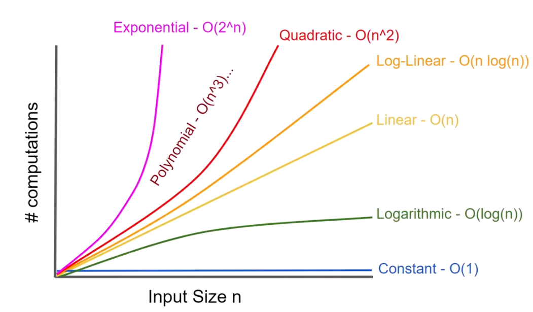
As the graph illustrates:
- O(1) and O(log n) are extremely efficient and scalable, as their resource consumption barely increases with input size.
- O(n) and O(n log n) are also considered very good and are common for efficient algorithms that need to process every element.
- O(n²) (Quadratic) and higher-order Polynomial complexities show a significant curve, indicating that they can become costly as the input size grows.
- O(2ⁿ) (Exponential) demonstrates an explosive growth rate, quickly becoming computationally infeasible even for moderately small input sizes.
| Complexity | Name | Explanation & Analogy | Code Example |
|---|---|---|---|
| O(1) | Constant | The algorithm takes the same amount of time regardless of the input size. Analogy: Picking the first apple from a basket. | int getFirst(int[] arr) { return arr[0]; } |
| O(log n) | Logarithmic | The algorithm’s time increases very slowly as the input size grows. It works by repeatedly halving the problem space. Analogy: Finding a word in a physical dictionary. | Binary Search |
| O(n) | Linear | The time taken grows linearly with the input size. Analogy: Reading every page in a book. | for (int x : arr) { ... } |
| O(n log n) | Linearithmic | A common complexity for efficient sorting algorithms. It scales well. Analogy: Sorting a deck of cards using merge sort. | Merge Sort, Quick Sort |
| O(n²) | Quadratic | The time taken grows exponentially with the input size. Often involves nested loops. Analogy: Checking if any two people in a room have the same birthday. | for (int x : arr) { for (int y : arr) { ... } } |
| O(2ⁿ) | Exponential | The time taken doubles with each new element added to the input. Becomes unusable very quickly. Analogy: Trying every possible combination to crack a password. | Recursive Fibonacci calculation |
| O(n!) | Factorial | The time taken grows extremely fast. Often involves finding all permutations of a set. Analogy: Finding the optimal travel route visiting every city once (Traveling Salesman Problem). | Finding all permutations of a string |
How to Calculate Complexity: A Practical Guide
Calculating Big-O complexity doesn’t have to be hard. Follow these simple rules:
- Drop Constants: An algorithm that takes
2nsteps is simplified toO(n). We only care about the growth rate. - Drop Non-Dominant Terms: An algorithm that takes
n² + nsteps is simplified toO(n²). The fastest-growing term dominates for large inputs. - Sequential Loops Add: If you have two separate loops, you add their complexities.
O(n) + O(m). - Nested Loops Multiply: If you have a loop inside another loop, you multiply their complexities.
O(n * m).
Example Analysis:
void processData(int[] numbers, String[] names) {
    // Rule 1: This is O(n) where n is numbers.length
    for (int number : numbers) {
        System.out.println(number);
    }

    // Rule 3: This is O(m) where m is names.length
    for (String name : names) {
        System.out.println(name);
    }

    // Total complexity for sequential loops: O(n) + O(m) -> O(n + m)

    // Rule 4: Nested loops multiply
    for (int number : numbers) { // O(n)
        for (String name : names) { // O(m)
            System.out.println(number + name);
        }
    }
    // Total complexity for nested loops: O(n * m)
}
Complexity Cheat Sheets
Common Data Structure Operations (Worst Case)
| Data Structure | Access | Search | Insertion | Deletion |
|---|---|---|---|---|
| Array | O(1) | O(n) | O(n) | O(n) |
| Stack | O(n) | O(n) | O(1) | O(1) |
| Queue | O(n) | O(n) | O(1) | O(1) |
| Linked List | O(n) | O(n) | O(1) | O(1) |
| Hash Table / Set | N/A | O(1)* | O(1)* | O(1)* |
| Binary Search Tree | O(n) | O(n) | O(n) | O(n) |
| AVL Tree / B-Tree | O(log n) | O(log n) | O(log n) | O(log n) |
| Heap | O(n) | O(n) | O(log n) | O(log n) |
Note: The O(1) complexity for Hash Tables and Sets represents the average case. Their widespread use is due to this performance. The theoretical worst case is O(n), which occurs in the rare event of widespread hash collisions.
Common Sorting Algorithms
| Algorithm | Best Case | Average Case | Worst Case | Space Complexity |
|---|---|---|---|---|
| Bubble Sort | Ω(n) | Θ(n²) | O(n²) | O(1) |
| Insertion Sort | Ω(n) | Θ(n²) | O(n²) | O(1) |
| Selection Sort | Ω(n²) | Θ(n²) | O(n²) | O(1) |
| Heap Sort | Ω(n log n) | Θ(n log n) | O(n log n) | O(1) |
| Merge Sort | Ω(n log n) | Θ(n log n) | O(n log n) | O(n) |
| Quick Sort | Ω(n log n) | Θ(n log n) | O(n²) | O(log n)* |
Note: Quick Sort space complexity can be O(n) in the worst case.
Resources & links
Articles
-
The Ultimate Guide to Complexity Analysis (Medium)
A comprehensive guide covering asymptotic notations (Big O, Omega, Theta) and illustrating common time and space complexities with Java code examples.
-
Algorithmic Complexity (Devopedia)
A detailed look at how complexity measures an algorithm’s execution time relative to its input size, with explanations of the different notations and complexity classes.
-
Complete Guide On Complexity Analysis (GeeksforGeeks)
An in-depth guide from GeeksforGeeks covering all facets of complexity analysis, from notations to measuring and optimizing time and space complexity.
Videos
-
Learn Big O notation in 6 minutes (Bro Code)
A quick and energetic introduction to the main concepts of Big O notation, perfect for a first look or a quick refresher.
-
Algorithms Explained: Computational Complexity (DataDaft)
A clear, animated video that explains the fundamentals of computational complexity and how it’s used to classify algorithms.